Graph - Pie section

A pie graph section displays data as slices of a circle, where each slice represents a proportion of the whole. Pie graphs are ideal for showing relative proportions and percentages of different categories or fields at a specific point in time or over a time period.

important

For pie graphs, you must use aggregation functions to return exactly one value per field. Without aggregation, the query would return multiple data points, which cannot be displayed as a single pie chart.

For pie graphs, you need a query that returns:

• Multiple fields or categories (each becomes a slice of the pie)
• One aggregated value per field (SUM, AVG, MAX, MIN, etc.)
• Typically covers a time range but returns a single summarized value for each field

The size of each pie slice is proportional to its value relative to the total of all values.

For more info on how to write queries, check the query differences for database and query examples

Basic example - Average over time period

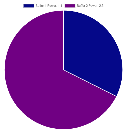
This example calculates the average power consumption for two buffers over a time period. Each field becomes one slice of the pie, showing the relative proportion of power usage.

SELECT 
  MEAN("InputBuffer1_PowerKw") AS "Buffer 1 Power",
  MEAN("InputBuffer2_PowerKw") AS "Buffer 2 Power"
FROM "oneWeek"."Line1"
WHERE time >= '2026-05-03T10:00:00+02:00'
  AND time < '2026-05-03T11:00:00+02:00'

SELECT 
  AVG("inputbuffer1_powerkw") AS "Buffer 1 Power",
  AVG("inputbuffer2_powerkw") AS "Buffer 2 Power"
FROM "docsdemo_timescale_wide"."line1"
WHERE time >= '2026-05-03 10:00:00+02'
  AND time < '2026-05-03 11:00:00+02'

WITH wide_data AS (
  SELECT
    AVG(CASE WHEN name = 'InputBuffer1_PowerKw' THEN value END) AS buffer1,
    AVG(CASE WHEN name = 'InputBuffer2_PowerKw' THEN value END) AS buffer2
  FROM "line1"
  WHERE time >= '2026-05-03 10:00:00+02'
    AND time < '2026-05-03 11:00:00+02'
    AND name IN ('InputBuffer1_PowerKw', 'InputBuffer2_PowerKw')
)
SELECT
  buffer1 AS "Buffer 1 Power",
  buffer2 AS "Buffer 2 Power"
FROM wide_data

Total consumption comparison

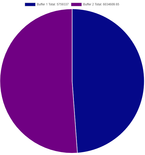
This example uses SUM to show the total energy consumption for each buffer over a time period, making it easy to compare which buffer consumed more total energy.

SELECT 
  SUM("InputBuffer1_PowerKw") AS "Buffer 1 Total",
  SUM("InputBuffer2_PowerKw") AS "Buffer 2 Total"
FROM "oneWeek"."Line1"
WHERE time >= '2026-05-03T00:00:00+02:00'
  AND time < '2026-05-04T00:00:00+02:00'

SELECT 
  SUM("inputbuffer1_powerkw") AS "Buffer 1 Total",
  SUM("inputbuffer2_powerkw") AS "Buffer 2 Total"
FROM "docsdemo_timescale_wide"."line1"
WHERE time >= '2026-05-03 00:00:00+02'
  AND time < '2026-05-04 00:00:00+02'

WITH wide_data AS (
  SELECT
    SUM(CASE WHEN name = 'InputBuffer1_PowerKw' THEN value::numeric END) AS buffer1,
    SUM(CASE WHEN name = 'InputBuffer2_PowerKw' THEN value::numeric END) AS buffer2
  FROM "line1"
  WHERE time >= '2026-05-03 00:00:00+02'
    AND time < '2026-05-04 00:00:00+02'
    AND name IN ('InputBuffer1_PowerKw', 'InputBuffer2_PowerKw')
)
SELECT
  buffer1 AS "Buffer 1 Total",
  buffer2 AS "Buffer 2 Total"
FROM wide_data

Peak values comparison

This example uses MAX aggregation to compare the peak (maximum) values reached by each field, showing which buffer had the highest peak consumption.

SELECT 
  MAX("InputBuffer1_PowerKw") AS "Buffer 1 Peak",
  MAX("InputBuffer2_PowerKw") AS "Buffer 2 Peak"
FROM "oneWeek"."Line1"
WHERE time >= '2026-05-03T10:00:00+02:00'
  AND time < '2026-05-03T11:00:00+02:00'

SELECT 
  MAX("inputbuffer1_powerkw") AS "Buffer 1 Peak",
  MAX("inputbuffer2_powerkw") AS "Buffer 2 Peak"
FROM "docsdemo_timescale_wide"."line1"
WHERE time >= '2026-05-03 10:00:00+02'
  AND time < '2026-05-03 11:00:00+02'

WITH wide_data AS (
  SELECT
    MAX(CASE WHEN name = 'InputBuffer1_PowerKw' THEN value END) AS buffer1,
    MAX(CASE WHEN name = 'InputBuffer2_PowerKw' THEN value END) AS buffer2
  FROM "line1"
  WHERE time >= '2026-05-03 10:00:00+02'
    AND time < '2026-05-03 11:00:00+02'
    AND name IN ('InputBuffer1_PowerKw', 'InputBuffer2_PowerKw')
)
SELECT
  buffer1 AS "Buffer 1 Peak",
  buffer2 AS "Buffer 2 Peak"
FROM wide_data